Prj145 - BBB LX9 C++ and VHDL (Part5)

With a FPGA board and JTAG tools to load an image, the next step is to actually develop and use a VHDL application.  Since much of the VHDL is custom to the daughter board I focused on trying to get a basic digital control interface (BDC) that I could use with different daughter cards.  This has the added benefit of testing out the BBB-Fboard SPI and providing another set of GPIO ports.  The effort includes both the C++ and VHDL sides.  The following is a conceptual organization of the software.

C++ and VHDL Organization

The Fboard software primarily provides an interface to read and write the SPI interface to the Fboard hardware.  There are different flavors of SPI access including 8 and 16 bit accesses.  A device tree is installed and determines how the SPI interface is access – via the BBB sysfs interface or a PRU0 image.  The PRU0 is significantly faster and drives the SPI at multiple MHz while the sysfs version is on the order of kilohertz and is easier to start debug and test with.  The intent is that PRU1 can be used to issue SPI commands to PRU0 for application specific streaming of high speed data.

The basic digital control block (BDC) can be included in any FPGA image and provides a register interface via the SPI link between the BBB and the Fboard.  The control block is based on previous efforts and looks a lot like the Prj 141 digital interface.  The difference is that I wanted to simplify the programming model and allow each access to specify the register rather than needing a register access to control a selector for the next access to get to the target register.  A basic block diagram is below.

VHDL ControlBlock Implementing Basic Digital Control Interface

Each control block contains a set of 8 bit read/write registers, some 16 bit counters, and two GPIO units.  Registers/counters can be added with each bit or set of bits interfacing with other application specific VHDL logic. Each GPIO unit has three registers (one for input, output, and direction of pins). The GPIO units connect directly with each of the 10 pin ports on the Fboard. Each of these registers has its data and read/write valid signals muxed based on a register id from a finite state machine.
This state machine conducts the read/write of a register based on an SPI command.  The finite state machine has a register fifo with a 16 bit SPI slave.  The state machine to process SPI commands operates at 96MHz (8x the XO on the F board using a DCM) and takes multiple clocks to read or write a register.

The SPI interface timing is specified to support a 20MHz SPI clock (for FPGA timing and layout only, the BBB even with the PRU will not exceed 16MHz with 9MHz being more realistic).  The software is designed to clock 16 bits into the SPI register at the same time 16 bits are clocked out.  The format of a SPI word is below.
         -- Bit position
         -- 1111 1100 0000 0000
         -- 5432 1098 7654 3210
         -- RWNN NNNN VVVV VVVV
         -- Where:
         -- R = 1 => read
         -- W = 1 => write
         -- N = register selector
         -- V = 8 bit write value
The upper two bits select whether a read or write is conducted.  In both cases the next 6 bits identify the register to be operated on.  In the case of writes, the following 8 bits of value are written to the specified register.  In the case of a read, these 8 bits are ignored, and the specified register is read (16bits) and saved in an internal register.  On the next SPI access, while the new commands bits are being shifted in these 16 bits are being shifted out.

This might seem a bit counter intuitive, however, it keeps the finite state machine simple and extensible, focuses on single operation writes (8 bits of which is sufficient for my purposes) and allows streaming 16 bit reads with little overhead (e.g. for ADCs).  It also allows 2^6 = 64 registers to be defined. The first 15 registers are dedicated to common operations like: a) FPGA image and version identification, b) Debug counters, c) LED control/signaling, and d) the two GPIO ports.  The second set of 15 registers is dedicated to the application specific basics (for example the DDS frequency value).  A 16 bit read fifo is used as the last register available.

Related:

Prj 145 - Beagle Bone Black Simple LX9 FPGA board (Part 1)
Prj 145 - BBB LX9 FPGA Board Design (Part 2)
Prj 145 - BBB LX9 FPGA Board Construction (Part 3)
Prj 145 - BBB LX9 JTAG Boundary Scan Utilities (Part 4)
Prj 145 - BBB LX9 C++ and VHDL (Part5)

Prj145 - BBB LX9 JTAG Boundary Scan Utilities (Part 4)

Previous posts walked through the overview, schematic, and fabrication of a fpga board for mixed signal use with a Beaglebone Black.  This post summarizes the boundary scan tools used to load the fpga image.

The JTAG boundary scan (JTAG for short here after) along with the DONE, INIT, and PROGRAM_B pins are accessible via BBB GPIO pins.  There are two utilities used to provide key functionality with these pins.

JTAG Boundary Scan Tools for Beagelbone Black LX9 Board

The first is Fxvc which is a virtual cable daemon based on software from Xilinx and tmbinc. This utility allows the Xilinx tool set to program and interrogate the fpga without a hardware cable. Within iMPACT, you select a loadable module under cable setup and supply:

xilinx_xvc host=192.168.0.2:2542 disableversioncheck=true

The tool then uses the network connection to conduct all JTAG operations.  The code is factored into two components: the general server which handles network transactions and the board specific portion which turns JTAG operations into pin level settings.  The tool was developed using a JTAG device simulator and was actually a really insightful exercise in understanding JTAG boundary scan.

The second tool is Fxsvf which is an embedded SVF player.  SVF is a way to express JTAG operations in a text file, while XSVF is a Xilinx binary form of SVF which results in more compact files.  Again, the application is broken into two components, a portion which handles the reading and parsing of an XSVF file and a portion which is board specific and sets the JTAG pins appropriately. The general part comes from the Xilinx XAPP058.  Due to licensing, this portion is currently not open source and can only be obtained by registering with Xilinx.  For this reason, the general XSVF player portion is treated as an installed library that you link the board specific pin manipulation code against to produce the final application.

One of the down sides to the current approach is the performance.  Manipulating GPIO pins from user space with the sysfs interface is quite slow (but simple).  I knew this going in but underestimated the convenience of being able to just attach to the fpga JTAG interface by running an application and having an Ethernet connected (which is always the case for my BBB work).  Not having to drag out yet another cable is really nice.

One of the issues I encountered was getting the ISE 14.7 tools to properly program the flash.  This process is what Xilinx calls indirect programming.  It involves loading a fpga image via JTAG that can manipulate the flash SPI pins via the JTAG interface.  This would not work for me.  At first I suspected a problem with my layout of the flash SPI, then I suspected a fabrication error, then I investigated Fxvc errors.  Eventually I ended developing my own utility Fflash to access the SPI flash and found no problems.  I found a couple of data points indicating the ISE tools sometimes have issues with SPI flash access (e.g. my identical issue - ID check failing, however, the workaround failed to solve my problem).  Given this along with the support state of ISE, I decided to abandon this approach and just work with my own flashing utility.  This is less of an issue than I first thought since my general use model is to load an FPGA image with iMPACT while debugging and then once the image is finalized save a copy and flash it.

The process involves first loading via Fxsvf a fpga image which directly connects the host SPI pins to the flash SPI pins. The Fflash utility then programs the SPI flash using the host SPI lines.  When using the PRU interface to the host SPI pins this is extremely fast - about 3 seconds to erase the device (device limited) and less than a second to program and verify the image into the flash.

Related:
Prj 145 - Beagle Bone Black Simple LX9 FPGA board (Part 1)
Prj 145 - BBB LX9 FPGA Board Design (Part 2)
Prj 145 - BBB LX9 FPGA Board Construction (Part 3)
Prj 145 - BBB LX9 JTAG Boundary Scan Utilities (Part 4)
Prj 145 - BBB LX9 C++ and VHDL (Part5)

Prj 145 - BBB LX9 FPGA Board Construction (Part 3)

This post captures a few notes on the fabrication of a BeagleBone Black minimal FPGA board. Previous posts covered the block diagram and schematic.  The board is a 2 layer OSH Park order at roughly 3" x 2".  One of the differences with this board is that I used 0603 resistors and capacitors for density reasons rather than 0805's I normally use.  I have used these in the past in a limited capacity.  The mechanics of mounting these are no different, however, I did find that the smaller parts slowed me down.  In the end, I think it was worth it as there were a couple of places where the 0805's would have made the board layout more difficult. Beyond the this, and the TQG package, there is nothing too challenging about this build.

Spartan 6 LX9 Board.

LX9 Board Mounted to Beagel Bone Black

This was the first time I had used a TQG package, so I was a little nervous about how it would turn out.  I have gotten reasonably good at working with 0.5mm pitch QFNs but only in the 40 pin range. Airgunning the QFNs works really well and they self align nicely if you get the solder paste application right.  I only have a jewelers loop not a microscope so manual alignment was a concern. My attempt on the first version of this board used an airgun.  This was not a good idea.  The problem with this is the shear area - its 22mm X 22mm.  It took forever to get the paste to melt and I had a hard time evenly distributing the hot air around the perimeter of the part.  There are hoods for air guns (which I do not have).  The board above used manual placement with a soldering iron.  I tacked down a pin on one corner, inspected, and then tacked down a pin on the opposing corner.  This was followed up with running a solder bead down each side and then wicking off the excess solder (you can see the flux residue from this around the part).  This worked out extremely well and was simple to do.  The picture below captures a closeup of the end result.

Closeup of hand soldering and alignment of TQG-144.

The only issue with the technique is that if too much solder is applied it tends to walk up the knee of the pins where it creates shorts with adjacent pins.  This high in the knee makes it difficult to wick off. I found that inspecting all of the pins from three different angles (front on, top angled left, and top angled right) allowed me to catch all instances of this.

Related:
Prj 145 - Beagle Bone Black Simple LX9 FPGA board (Part 1)
Prj 145 - BBB LX9 FPGA Board Design (Part 2)
Prj 145 - BBB LX9 FPGA Board Construction (Part 3)
Prj 145 - BBB LX9 JTAG Boundary Scan Utilities (Part 4)
Prj 145 - BBB LX9 C++ and VHDL (Part5)

Prj 145 - BBB LX9 FPGA Board Design (Part 2)

This post summarizes the schematic of a BeagleBone Black FPGA board (overview and block diagram).  This is a minimal FPGA board intended for use with ADCs and DACs so it does not include complicating aspects like DRAM, HDMI, or high speed serial.  Having said this, Xilinx UG-380 does a good job describing the JTAG boundary scan interface, SPI flash interface and configuration interfaces (done, program_b, M0, M1).  You just have to read and study it quite a bit.  The only subtle aspect is the power-on/reset sequencing.

I wanted to use the +5V directly from the unregulated BBB input to allow for higher current draw of this board and daughter boards.  The power on sequence of the LX9 is well defined with high-Z IO pins.  It is the reset and shutdown sequence that has to be addressed.  In this scenario, the BBB and the FPGA board can be powered on, loaded, and operating normally when the user provides a shutdown command to the BBB linux which disables the on board regulated supplies but leaves the +5V unregulated input on (i.e. the wallwart is plugged in but a shutdown has been issued and the BBB is off).  In this case, the LX9 could be left powered up, configured and driving the SPI and JTAG pins while the ARM on the BBB is powered off.  To avoid this problem and allow use of the unregulated supply, a high side switcher is used to control the +5V with the enable being the BBB 3.3V regulated supply.

There are 32 IO pins at one edge of the board with a ground every 4 pins.  The very end provides +5 with 4 pins.  This nicely fits within a 2x23 header (the same used by the BBB).  Since additional pins are available those are brought out to two 2x5 headers.  These are the same used on the I board and include +5V power.  This allows interfacing with other boards using a low speed SPI or I2C.

Schematic Page 1 - LX9, Connectors, Flash, Clock.

Schematic Page 2 - Power and Bypass Capacitors

Screenshot of PCB Layout

The KiCad source material along with pdf of schematic and zip of Gerbers is available here.

The overall cost sourcing from OSHPark and Digikey is $12 for the PCB (quantity 3), LX9 $18 (quantity 1), connectors $3, oscillators, and regulators $3,  Flash and passives $3 for a rough total of $39 per board.

Related:
Prj 145 - Beagle Bone Black Simple LX9 FPGA board (Part 1)
Prj 145 - BBB LX9 FPGA Board Design (Part 2)
Prj 145 - BBB LX9 FPGA Board Construction (Part 3)
Prj 145 - BBB LX9 JTAG Boundary Scan Utilities (Part 4)
Prj 145 - BBB LX9 C++ and VHDL (Part5)

Prj 145 - Beagle Bone Black Simple LX9 FPGA board (Part 1)

One of my objectives is still to have a simple and low cost FPGA board to use with an ADC or DAC of intermediate sampling rate (10MSPS – 60MSPS).  There are a number of good off the shelf FPGA boards available to support this (for instance).  After looking at several I kept coming back to the concern that the I/O configuration was just a little less than optimal for what I wanted to do.  For me, I only need one or two FPGA boards, while I pay per square inch for each analog board.  If the headers are wide and offset, then it takes another 3x2 inches I do not really need just to mate the analog and FPGA board.  This then ends up costing 6sq. inches x $5/sq. inch for each analog design in dead area. Said differently, if I could just get the I/O in a slightly different configuration… (this appears to be a costly and slippery slope akin to telling yourself that your current house would be just fine if you only had one more room).

Given the IO desire and a better understanding of what could fit in a Spartan6 LX9 along with what I did and did not require for additional hardware, I decided to try a minimalist hand solderable FPGA board.  The LX9 is the largest part available in a TQG-144, beyond that its BGAs.  To keep things simple all of the IO is 3.3V with a minimal set.  There are 32 pins with a ground every 4 pins in a single header at one edge of the board.  A  SPI and JTAG boundary scan ports are at the other edge of the board.  This configuration allows the mounting on a BeagleBoneBlack and keeping analog daughter card growth at one end of the board.

Notional Board Stack Up of BBB, FPGA Board, and Mixed Signal Board.

Since there are plenty of IO pins (and in an accessible spot) there is also room to add 2 ports of 6 pin GPIO at the end of the board.  These would match the pin-out used in previous I board peripherals and include a +5V supply.  A few additional BBB GPIOs are needed to address the LX9 reset and control pins (DONE, INIT, PROGRAM_B).  A block diagram of the interface configuration is shown below.

BeagleBoneBlack-FPGA Board Interface

One of the key points is that the SPI interface is on BBB pins which are accessible via PRU0.  This is important since the PRUs can be used to obtain higher performance SPI interfaces than the built in hardware units (examples here, here, and here).  While the basic SPI is 4 pins (SCLK, SS, MISO, MOSI) an additional 2 pins were dedicated to provide a 2x SPI (i.e. MISO0, MISO1, MOSI0, MOSI1). I would dedicate more, however, there are virtually no more easily accessible PRU mappable GPIO pins available on P9.  P8 could be used, however, P9 has the +5V from the main power so this would require pins (and obstructions) on both ends of the FPGA board and subsequently the stacked mixed signal board.

Related:
Prj 145 - Beagle Bone Black Simple LX9 FPGA board (Part 1)
Prj 145 - BBB LX9 FPGA Board Design (Part 2)
Prj 145 - BBB LX9 FPGA Board Construction (Part 3)
Prj 145 - BBB LX9 JTAG Boundary Scan Utilities (Part 4)
Prj 145 - BBB LX9 C++ and VHDL (Part5)

Prj 141 - Spartan6 LX9, ADC, and BBB (Part1)

AdcHttpd - HTML5/Browser Based Signal Analysis Tool

As part of the X board/DDC efforts I decided to redo the adc tool I was using.  The original set used a java application on the PC and a server on the BBB.  The java application provided controls and presentation of the data and processing of the samples.  This worked fine but each time I went to take a measurement I needed the PC application.  There also seemed to be a lot of interface work in both the java client and on the server every time I wanted to make a small change (e.g. particularly for controlling the acquisition and hardware configuration).  Previous experiments with javascript/browsers indicated that network and processor performance and loading would be sufficient to support the intended use.  There are two advantages to this approach in my mind: a) there is no client application, just a browser and b) the interfacing software is simpler and better localized by using JSON which provides good support for serialize/deserialization with javascript software and is easy to produce/parse within a C++ application.

The following image shows the browser presentation.

Chrome with AdcHttpd on a BeagleBone Black with 16 bit DDC data from a LX9

The main area is a HTML5 canvas which is drawn using a basic graphing toolkit I developed for instrumentation purposes.  The buttons at the bottom are HTML buttons with javascript actions.  The first row allows presentation changes (envelope, peak picking, user markers, storing a memory, changing Y limits).  The second row controls server side parameters such as the function to perform, in this case PSE or power spectral estimation, the number of points to produce, the number of averages to use, the channel to select and the LO frequency used in down conversion.  The channel is the tap point referenced in the DDC.  The final row sets the state to run or not run, or resets  various pieces of software.  The line above the graph also includes key parameters in effect along with the date and status of the connection to the http server (it turns red and indicates not connected if a threshold of failed server requests is reached).

The numeric quantities that are free form input (e.g. F1(Hz) or LO mixer or the upper and lower graph limits) are entered via a javascript keypad.  The following screen capture shows the same channel or signal as the previous capture but this time in the time domain and with the keypad popped up to modify the Y limits.

Javascript Keypad Input (Time series in background of signal in previous figure)

The browser tab consumes about 10% of a CPU core on an older PC (AMD 1.8GHz quad core) and about 1% load on the Ethernet interface.  The BeagleBone is at 98% running the http server.  The BBB limits the update rate based on its ability to process the samples (fftw for ARM is used for best performance).

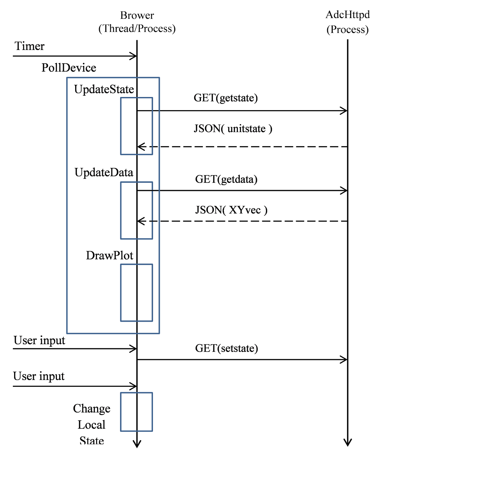
There are several components to the internals of the browser code, http server code, hardware model, and device code on the BeagleBone Black.  The basic model is that the server is the definitive controller of state and operations while the browser code simply requests changes and conducts presentation.  At the highest level the following sequence diagram summarizes the interactions of the application.

Browser-AdcHttpd Summary Sequence Diagram 

The Browser lifeline captures the javascript code behavior executing within the browser while the AdcHttpd lifeline captures the software executing on the BeagleBone Black.  There are only two events handled by the javascript code: a timer and user input.  The timer forces a sequence of events which boil down to getting state and data from the server and drawing a plot of the current data.  All information is obtained from the server via http GET requests.  The results coming from the server are JSON text representing application variables.  The diagram is slightly off in that the responses coming back are processed asynchronously to the request.  There is additional logic to keep the state requests at a lower request rate than the requests for data.  In addition, there is logic to adjust the polling rate based upon the operational state of the instrument.  Quantities in the overall state include things like channel number to process, run/stop state, mixer frequency.  The data coming from the server is just a x,y list of points to be plotted on the graph.

The other events processed by the browser javascript are user inputs.  This ends up taking two forms: a) those which change server state and are sent directly to the server, and b) those which change local browser application state and can be processed without interaction with the server.  Examples of the former include run/stop state or channel number and examples of the later include graphing x and y limits, peak picking enable/disable, and markers on/off.

The server is more involved and is responsible for not only acquiring the data and processing it but also presenting it in JSON format to the client.  The following sequence diagram summarizes the key server components and interactions.

Summary Sequence Diagram of AdcHttpd Internals

There are only two autonomous lifelines here by design.  The first is the http server thread that interacts directly with the client and processes the http GET requests.  The second is the hardware model thread which drives processing of data and hardware interactions.  The only point the two threads interact is the hardware data model.  The interactions are designed to require minimal locking and interaction between the two autonomous threads.  This keeps things conceptually simple and decouples the browser client and its interactions and requests from the core hardware servicing and operations.  The hardware object model contains the current and desired operation parameters along with the most recent XY data to be presented in the browser application.

The hardware model thread checks various operating parameters based on their current value in the memory shared with the http thread.  If changes have occurred, the hardware model thread calls the appropriate device object methods to change the operating parameters.  Examples include which channel is being processed/exported by the hardware and the frequency of the downconversion local oscillator.  After a check on current parameters the hardware model thread invokes the ProcessCoherentInterval() on one of the processing objects.  There are processing objects for each of the main types of processing: power spectral estimation, time series, and histogram.  The product of processing a coherent interval is a set of XY points which is updated in the hardware model (and can then be accessed by the remote client via the main http thread). The hardware model thread continually loops on this processing until a reset is conducted.

Each of the processing objects deals with a coherent interval a little differently.  The key one is the power spectral estimation processing.  Since the data rates of the selected ADC channel can exceed the processing capability (indeed the network transport capacity), a processing interval is treated as a flush of current ADC data followed by the acquisition of one or more sets of 2k samples.  The collected data is treated as a coherent set and in the case of spectral estimation has a window applied along with an FFT and magnitude and normalization applied to produce the XY results.  In the case of low sample rate channels, 16k or more samples can be treated coherently since successive Get2k calls retrieves contiguously sampled data.  For streams with high bandwidth, the user simply has to not configure power spectra estimates greater than 2k (if you do you just get phase discontinuities across 2k sample sets and see spectrum broadening).

The device object encapsulates different boards.  There are a common set of C++ ADC and Mixer interfaces required that each board exports.  The startup method for the device object selects which boards and interfacing software to use.  This can be done by configuration file, code  changes or reasoning on which device tree(s) are currently installed.

Prj 141 - DDC at 60MSPS (Part 8 - Final)

This if the final post walking through a digital down converter and ADC on a Beaglebone Black (Part1, Part2, Part3, Part4, Part5, Part6  and Part7).

All of the previous work was conducted with a 10MSPS clock and ADC.  The next step was to increase to 60MSPS.  The only changes required were updates to the DDC filters.  Due to the increased decimation some of the internal paths experienced bit growth and needed to be widened.  The internal test pattern generation capability within the fpga image allowed this to be worked through all of these changes.

Everything worked fine until an actual signal was applied.  At that point I had problems with digital values being read twice.  This shifts the IQ values by one every now and then which destroys the quadrature relationship. The transfer rate across the IDC was 100k samples per second with each sample being 16 bits.  The transfer rate (or down converted bandwidth) was dropped below 50kSPS which still did not fully rectify the problem.  Based on numerous experiments and trial and error I think the single ground pin (looking seen in schematics in this post) is causing problems with the SPI port voltage level sensing.  Using a single ground is a bit much to ask, I’m using the FPGA board in ways it was not designed for.  I believe that as the digital pins begin switching (changing ADC values) the current required through the ground pin increases.  A small residual resistance on the ground return with a large current can push the ground reference at the FPGA up.  This results in a lower voltage across the SPI digital inputs (i.e. between the IO pin input from the SPI clock or slave select to the FPGA ground reference value).  The final confirmation of this was getting error free results with the internally generated test pattern with an open analog input but the same setup began generating errors when a simple wire antenna was attached to the input.  I contemplated using a differential converter at the SPI headers but decided against it as I suspected additional problems at this sample rate and a single ground through 0.1 headers.

This project was a great non-trivial introduction to VHDL and could be broken up into purchased pieces (XuLA2) and simple unique analog designs (ADC board).  At this point I'm going to have to contemplate my options for alternate approaches.

Related:
Prj141 Schematic
Prj141 Overview
Prj141 Digital Down Converter
Prj141 Digital Interface
Prj141 Software
Prj141 Filter Design
Prj141 Filter Evaluation
Prj141 LX9 Utilization
Prj141 Higher Sampling Rates